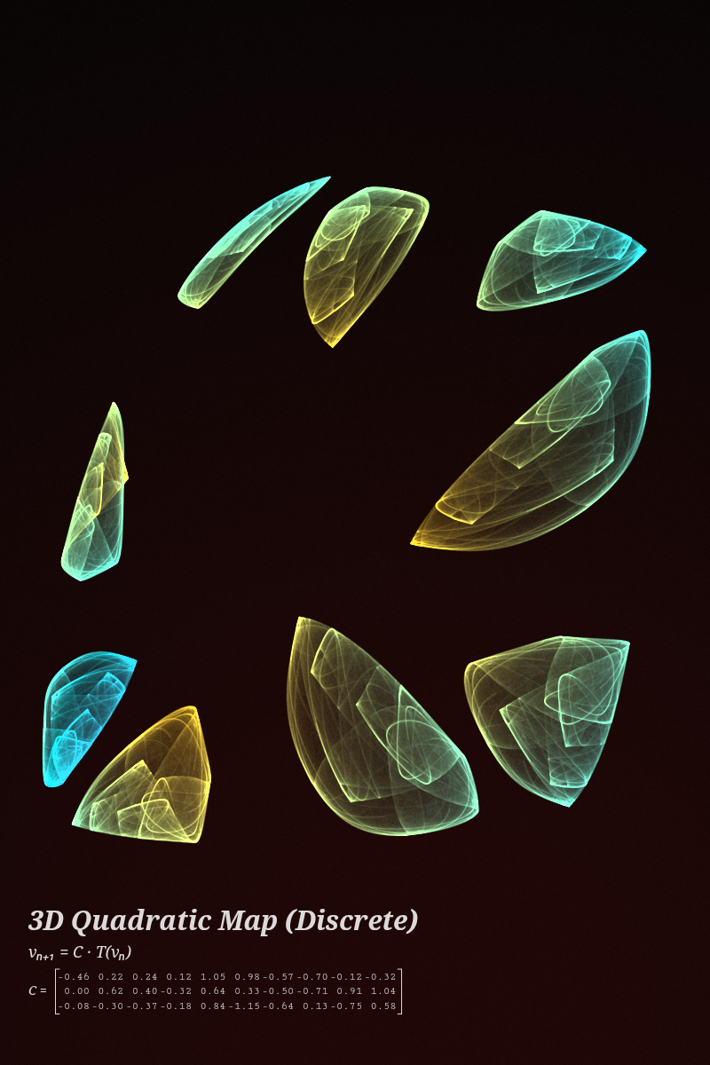
Discrete Iterated Map First Described: 1993

3D Quadratic Map (Discrete Iteration)

Discovered by J.C. Sprott & Chaos Explorers

Executive Summary

Crumpled gossamer membranes and multi-sheet fractal sheets generated by iterative 3D quadratic mappings.

System of Equations

Phase Space Formulation
xn+1=a0+a1xn+a2yn+a3zn+a4xn2+a5xnyn+a6xnzn+a7yn2+a8ynzn+a9zn2x_{n+1} = a_0 + a_1 x_n + a_2 y_n + a_3 z_n + a_4 x_n^2 + a_5 x_n y_n + a_6 x_n z_n + a_7 y_n^2 + a_8 y_n z_n + a_9 z_n^2
yn+1=b0+b1xn+b2yn+b3zn+b4xn2+b5xnyn+b6xnzn+b7yn2+b8ynzn+b9zn2y_{n+1} = b_0 + b_1 x_n + b_2 y_n + b_3 z_n + b_4 x_n^2 + b_5 x_n y_n + b_6 x_n z_n + b_7 y_n^2 + b_8 y_n z_n + b_9 z_n^2
zn+1=c0+c1xn+c2yn+c3zn+c4xn2+c5xnyn+c6xnzn+c7yn2+c8ynzn+c9zn2z_{n+1} = c_0 + c_1 x_n + c_2 y_n + c_3 z_n + c_4 x_n^2 + c_5 x_n y_n + c_6 x_n z_n + c_7 y_n^2 + c_8 y_n z_n + c_9 z_n^2

Governing Parameters

CC
Mapping Matrix (30 floats) = Discrete search space

Determines how coordinate space stretches, curls, and folds onto itself with each computational tick.

Overview

While continuous differential equations generate smooth, continuous ribbons and tubes, discrete maps operate through instantaneous algebraic transformations. At every iteration step nn+1n \to n+1, the point jumps across space according to a polynomial transformation rule.

In three dimensions, the general quadratic map folds 3D space like kneading dough: stretching coordinates along expanding eigenvectors, and folding them back along contracting directions. Over millions of iterations, points settle onto intricate fractal manifolds that exhibit self-similarity at all magnifications.

The Mathematical Framework

The recurrence relation is expressed vectorially as:

vn+1=CT(vn)\vec{v}_{n+1} = \mathbf{C} \cdot \vec{T}(\vec{v}_n)

where:

T(v)=[1xyzx2xyxzy2yzz2]T\vec{T}(\vec{v}) = \begin{bmatrix} 1 & x & y & z & x^2 & xy & xz & y^2 & yz & z^2 \end{bmatrix}^T

Distinctive Visual Character

  • Translucent Membranes: Because discrete iterations jump across space without drawing solid connecting curves, renderings look like diaphanous veils, planetary nebulae, or frozen smoke rings.
  • Cantor Dust & Fractal Cross-Sections: Slicing through any section of a discrete 3D attractor reveals a Cantor-like fractal dust of infinite complexity.
  • Extreme Parameter Space: The 30 coefficients define a vast mathematical universe containing billions of unique geometric species.
Previous Type
Polynomial Attractor (Sprott 3D System)
All Attractor Types
Next Type
Symmetric 3D Attractor